Forecasting Stock Prices Time Series Analysis (Excel: Moving Average, R: ARIMA)

May 2, 2022

Introduction

The objective of this analysis is to do the forecasting analysis on the price of two companies ( Costco Wholesale company (COST) and Coca-Cola (KO) from the previous 252 data period. Performing by using three separate forecasting models:

Exponential smoothing performed the short-term forecasting.
Weight moving average to complete the long-term forecasting for the following four periods.
ARIMA to make a long-term forecast for the next three months’ stock price and to forecast the wine price for the next ten years in the dry_wine.csv dataset.

Short-term forecasting

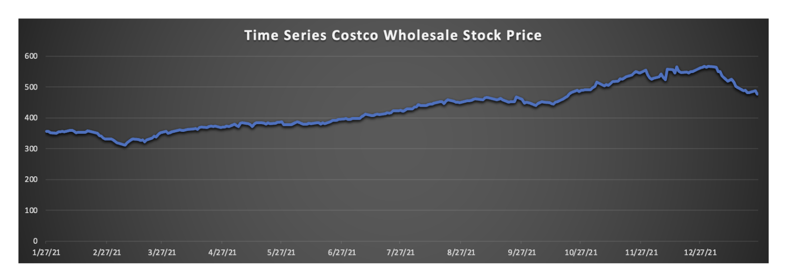
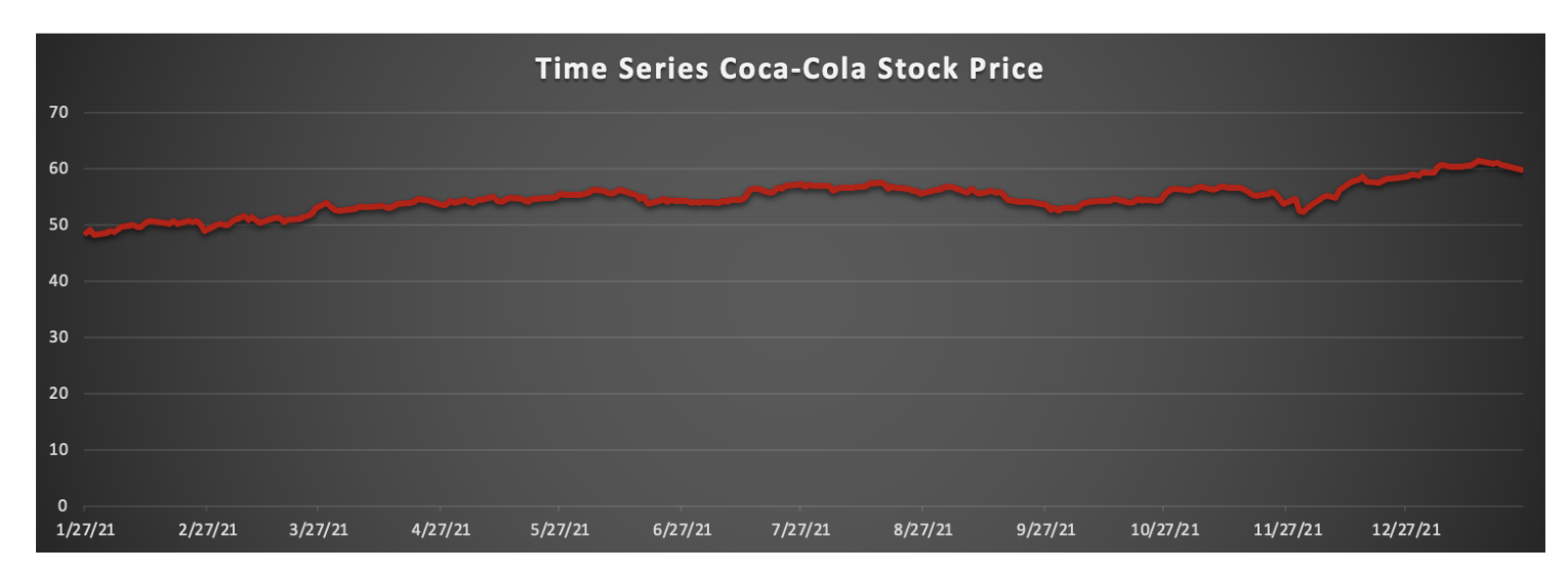
First, I examined the first preliminary property, which is the stationary check from the stock data we used to analyze. Both plots demonstrate a recurring pattern, implying seasonality. As a result, we can assume that this data is non-stationary. As a result, I employ the exponential smoothing model for the short-term forecast, which is one of the most efficient methods for forecasting non-stationary data.

To begin, I use exponential smoothing to anticipate the stock prices of Costco and Coca-Cola for the 253rd period, utilizing a range of successive alpha values (0.15,0.35,0.55,0.75) to determine which value produces the best forecast for our data.

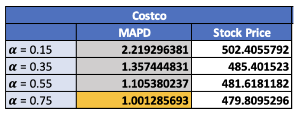
Based on our calculations, the final stock price in the 253rd period for alpha values of 0.15, 0.35, 0.55, and 0.75 is 502.4, 485.4, 481.6, and 479.8, respectively. According to the Mean Absolute Percentage Deviation (MAPD), a measure of how far projected data deviates from actual values. As expected, alpha = 0.75 produced the lowest MAPD, approximately 1.001. Therefore, we can assume that = 0.75 produces the best accurate forecasting data for the Costco stock price.

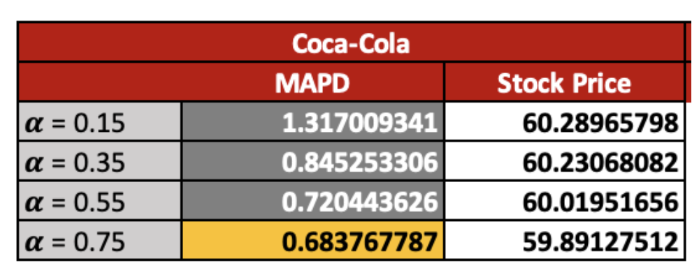
Following that, I used the same method to estimate Coca-253rd Cola’s stock price. As indicated by the MAPD of 0.68, the successive value that provides the most accurate results is 0.75. As a result, we can estimate that alpha = 0.75 effectively predicts the best stock price for the 253rd period, $59.89.

Next, I use the 𝜶 = 0.55 adjusted exponential smoothing approach to compare the output to the preceding method and determine which model delivers the most effective outcome, as well as the MAPE or Mean Absolute Percentage Error by using different trends successive values (0.15, 0.35,0.55 and 0.75).

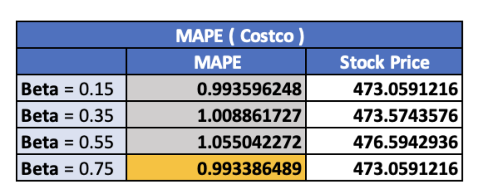
As a result, the Beta value that generates the most accurate forecasting for the Costco stock price is 0.75. By considering the MAPE values, which are only 0.99. On the other hand, for the Coca-Cola price prediction, the beta values that create the most efficient stock price is 0.15.

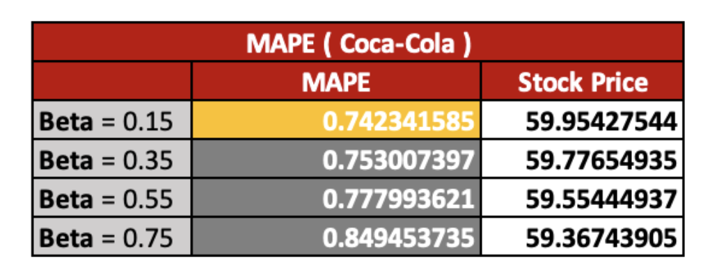
As a result, we conclude that the most effective successive trend values for Costco are 0.75, while the most effective successive trend values for Coca-Cola stock price predictions are 0.15.

Long-term forecasting

I applied the weight moving average to perform long-term forecasting to predict the Costco and Coca-Cola stock price for the 253rd-257th period and compare with the actual price that I retrieve from yahoo ( Yahoo, 2022 ). In order to determine the deviation of the forecasting price with the actual price.

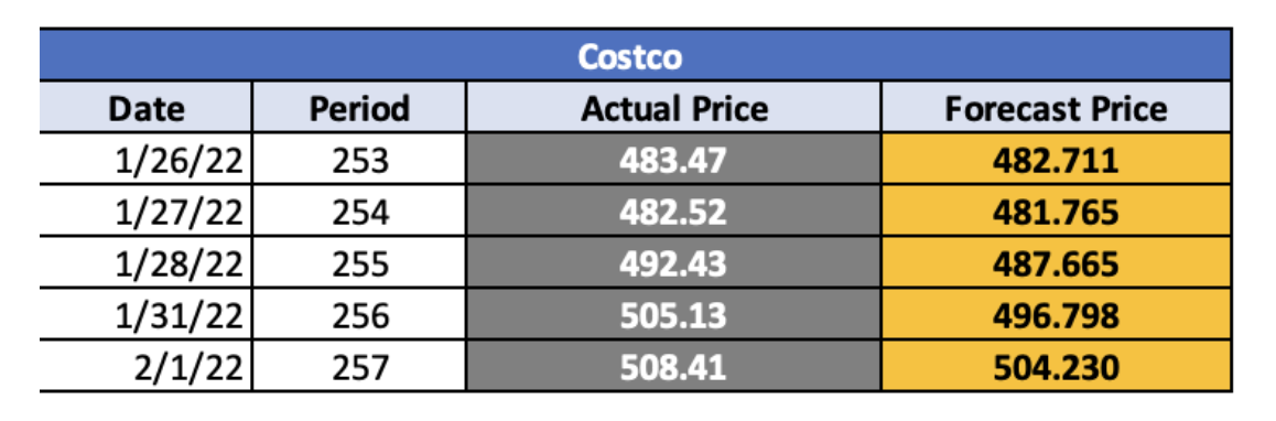
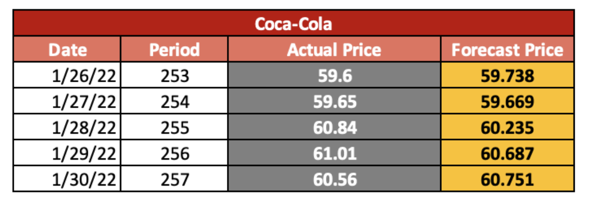
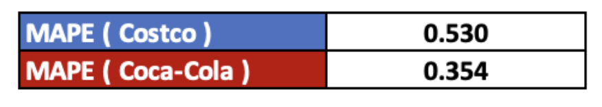
Based on the result of our prediction, we can see from Figures 7 and 8 that the forecasting price for both Coca-Cola and Costco is not much different from the actual value. We can ensure our prediction accuracy by using the MAPE to determine the percentage error from the actual value. Therefore, we can see that the MAPD indicates a very low deviation error from the actual price, which is 0.530% and 0.354% for the Costco and Coca-Cola price, respectively. Moreover, when we compare the MAPE of the long-term forecast with the short-term forecast, the result shows that the weight moving average generates a more accurate outcome than the exponential smoothing method. Therefore, in this case, I would suggest using the long-term forecast method

Time series analysis

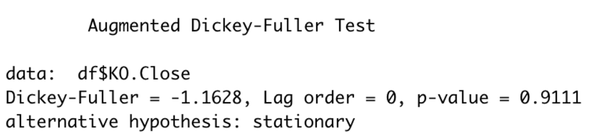
In this section, I forecast the Coca-Cola stock price for the next three months using a manual ARIMA model. To begin, I use the Augmented Dickey-Fuller Test in Figure 10 to determine whether the data is stationary or not. As a result of the significant p-value, we cannot reject the null hypothesis. As a result, we can infer that the data are non-stationary.

Since the data is non-stationary, the seasonal ARIMA is the best choice for our forecast. Next, I use the ACF and PACF as a reference to identify which model is the best suit for our forecast.

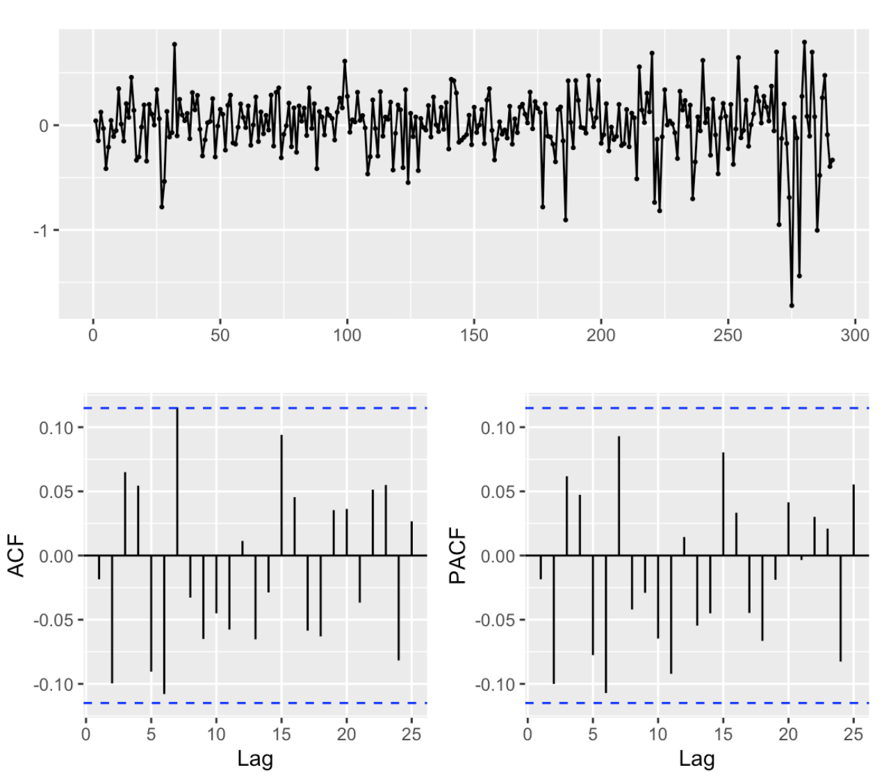
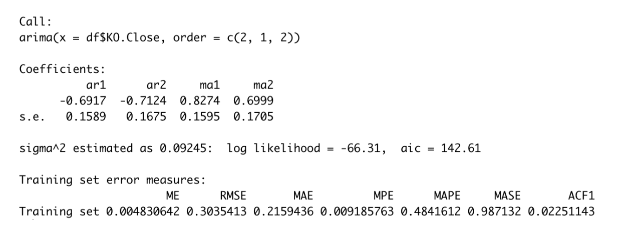
As illustrated in Figure 11, there is a substantial increase on lag 2, implying that the ACF supports a non-seasonal MA (2). Next, I compared AR(1) and AR(2) to see which model has the lowest AICc. Consequently, the model that generates the lowest AICc is ARIMA(2,1,2) with the AICc = 142.61.

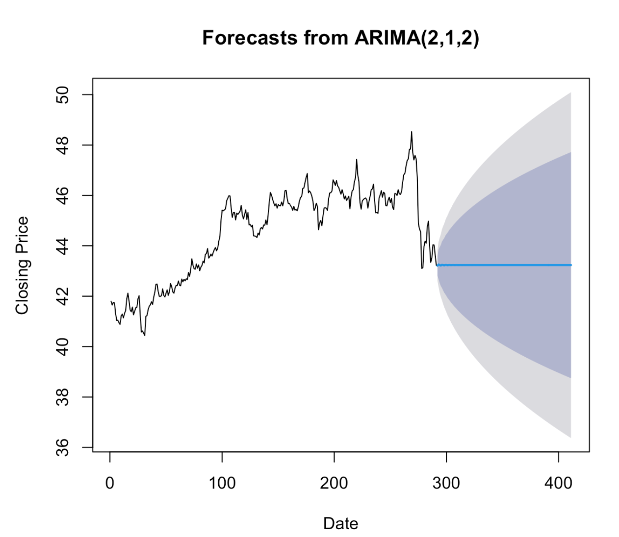
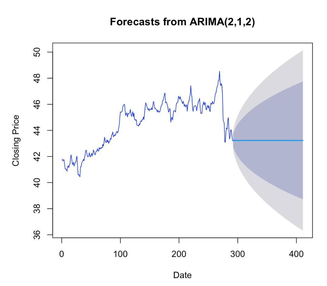
Finally, I forecast using ARIMA(2,1,2), the model that passes all the preliminary checks. The result indicates that the stock price will remain steady for the next three months, as indicated by the blue line, suggesting an average closing price of approximately 42. The shaded blue area denotes the forecast intervals that allow for both upward and downward trending of the data across the forecast period.

Additionally, I utilize the auto.arima method to confirm that my model selection is valid. According to the auto.arima result from Figure 14, the model we have chosen matches the model from our choice. As a result, this indicates that we have chosen the appropriate model.

Next, I applied the AR(1) for the manual ARIMA to compare the result with the auto.arima. But first, we need to do the preliminary check for the lag time to choose the best MA for our forecast.

According to Figure 15, the ACF and PACF both exhibit a rise in lags 1 and 2, showing that the ACF is compatible with a non-seasonal MA (1) and (2). As a result of applying ARIMA (1,1,1) and (1,1,2), the result suggests that ARIMA (1,1,1) produces a lower AICc than ARIMA (1,1,2). Therefore, in this case, I use ARIMA (1,1,1) for my forecast.

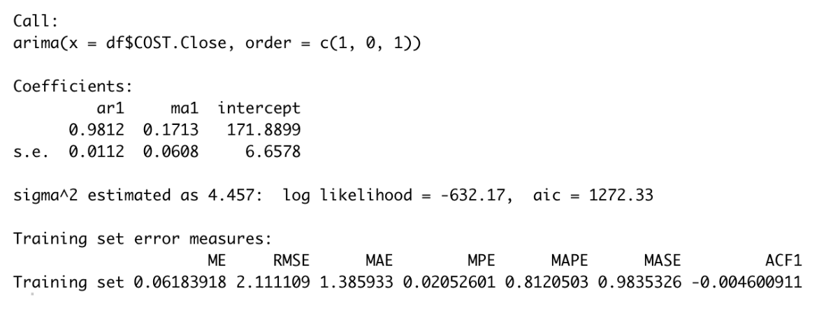
However, I would like to ensure that my option is the best possible. I compare the output of my manual ARIMA forecasting to the auto ARIMA forecasting generated by the program. The program suggests ARIMA(0,1,1), which provides the lower AICc (Figure 18), implying our calculation is not optimal. Therefore, I apply the ARIMA (0,1,1) to do the forecast.

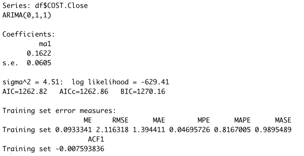
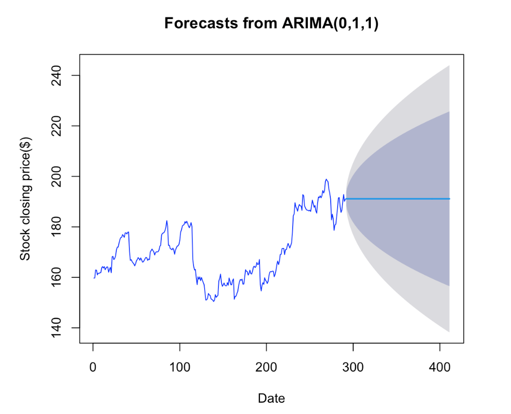
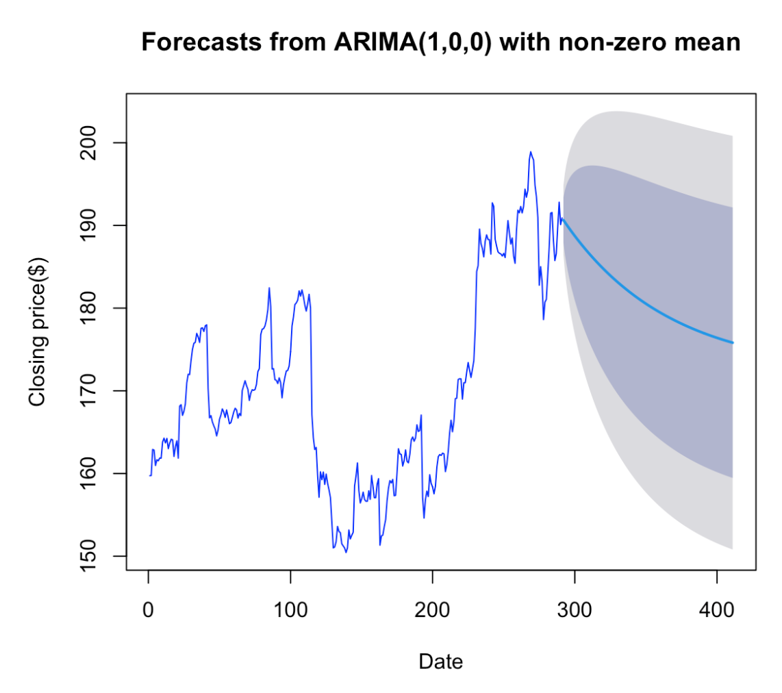
Our estimate predicts that the stock price will remain constant over the next three months, as represented by the blue line, implying an average closing price of about 190. The shaded blue region represents the forecast intervals that account for both upward and downward trending data across the forecast period.